House Price Prediction With Statistical Analysis in Support Vector Machine Learning for Regression Estimation

Introduction

In this paper, we explore the application of machine learning in predicting house prices. Specifically, we will be constructing a support vector machine for regression estimation. We attempt to improve model performance by implementing kernels for hyper-dimensional feature mapping We also go over statistical techniques commonly used in processing data for regression estimation. We find that there exists a trade-off between model complexity and performance. Should the model be either too simple or complex, we risk under-fitting or over-fitting the model. In between optimal model complexities, we find a trade-off between level of accuracy and general model performance. For a broader study of learning machines in house price prediction see Babb (2019).

The learning problem can be said to have started with Rosenblatt’s Perceptron (1962).^[1] Discoveries in learning theory, such as back-propagation (Bryson et al., 1963) for solving vector coefficients simultaneously (Le Cun, 1986) and regularization techniques for the overfitting phenomenon, have advanced understanding of the learning problem significantly. Since Rosenblatt’s digit recognition problem, the importance of statistical analysis in the learning problem has been emphasized greatly. The learning problem is that of choosing a function $f(x, \alpha)$, where $\alpha$ is a set of parameters, based on a set of independent and identically distributed observations that returns a value $\hat{y}$ most approximate to $y$. Hence, a supervised machine-learning model requires that in a set of observations $(x, y)$, $y$ is known a priori for training the model. A risk function $R(\alpha)=\int L(y, f(x,\alpha))dF(x,y)$, where $F(x, y)$ is the joint probability distribution function (pdf) of the observations, is used to measure the discrepancy $L(y, f(x,\alpha))$ between a learning machine’s output $f(x,\alpha)$ to a given variable $x$ and the observed value $y$. In this paper, we will consider the specific learning problem of regression estimation. In regression estimation, we wish to minimize the risk function $R(\alpha)$ with a loss function $L(y, f(x, \alpha)) = (y - f(x, \alpha))^2$.^[2] Of course, in order to minimize the risk function $R(\alpha)$ we must know the joint pdf $F(x, y)$. This is often not the case in real-world applications. Accordingly, the empirical risk minimization principle is applied to substitute the risk function with $R_e(\alpha) = \frac{1}{n} \sum_{i=1}^{n}(y_i - f(x_i, \alpha))^2$.

In 1992, Boser et al. proposed a training algorithm for optimal marginal classifiers. In 1995, Vapnik expanded this algorithm for regression estimation problems. Support vector machines (SVMs) are supervised machine-learning models that analyze data for classification problems. Such models can be modified for regression analysis with the use of logistic regression. SVMs have a complexity dependent on the number of support vectors rather than on the dimensions of the feature space (Vapnik, 1995); hence, SVMs are memory-efficient. Training data need not be linearly separable (though, this is an assumption made in the construction of optimal separating hyperplanes). We begin our inquiry by constructing a support vector machine without a hyper-dimensional mapping kernel. We will create additional models by implementing a polynomial kernel and the radial basis function (RBF). After running our dataset with each model, we will compare and contrast the results of their house price predictions.

In the following section, we introduce Vapnik and Chervonenkis’ (1974; cited in Devroye et al., 1996) optimal separating hyperplanes and the support vector learning machine used for constructing such hyperplanes. In Section 3, we introduce the dataset used and techniques in preparing the dataset for optimal model performance. Section 4 will go over techniques for creating and processing features to further improve model performance. We display and discuss the results in section 5. Finally, we make some concluding remarks in section 6.

Model Formulation

We begin by defining our training data of $m$ samples $(\textbf{x}_i,y_i)$, $i=1,2,\dots,m$, where $\textbf{x} \in R^n$ and $y \in R$; in other words, the variable vector consists of $n$ features and the output is a real value. A linear separating hyperplane has the form $\langle\textbf{w},\textbf{x}\rangle-b=0$, where the weight vector $\textbf{w}$ and the threshold scalar $b$ determine the position of the hyperplane. The optimal hyperplane is found by separating the variable vector $\textbf{x}_i$ into two different classes $y\in\{-1,1\}$ with the smallest norm $||w||$. This is done by minimizing the function

$$\phi(w)=\frac{1}{2}(w\cdot w)$$
subject to $y_i(\textbf{w}\cdot\textbf{x}_i-b)\geq1_i$ for $i=1,2,\dots,m$. The solution is found at the saddle point of the Lagrange function

$$G(w,b,\alpha)=\frac{1}{2}(w\cdot w)-\sum_{i=1}^m \alpha_i[|(\textbf{x}_i\cdot\textbf{w}-b)|y_i-1]$$
where $\alpha_i$ are the Lagrange multipliers. In the case that the data is not perfectly separable, we have penalties $\xi_i=max[0,1-y_i(\langle\textbf{w},\textbf{x}\rangle+b)]$. Here, to find the optimal hyperplane, we minimize

$$\phi(w,\xi)=\frac{1}{2}+C\sum_{i=1}^m \xi_i$$
where $C$ is a given regularization parameter, subject to $y_i(\textbf{w}\cdot\textbf{x}_i-b)\geq1_i-\xi_i$ and $\xi_i\geq0$ for $i=1,2,\dots,m$.

To account for non-linearly separable data, kernel tricks,^[3] originally proposed by Aizerman et al. (1964), are applied to map the vector $\textbf{x}$ to a high-dimensional feature space $Z$ (Boser et al., 1992). A kernel function simply replaces the inner products $\langle\textbf{x}_i,\textbf{x}_j\rangle$ with convoluted inner products $k(\textbf{z}_i,\textbf{z}_j).$ The result is a hyperplane in high-dimensional space that may or may not be linear in the original variable space. Consequently, the algorithms remain fairly similar and support vector machines are thus versatile and effective in high-dimensional spaces. We will create additional models by applying the inhomogeneous polynomial kernel function of degree $d$, defined $k(\textbf{z}_i,\textbf{z}_j)=(\langle\textbf{z}_i,\textbf{z}_j\rangle+r)^d$, where $r$ is a constant added to avoid problems with the inner product equalling 0 (specifically, we will consider degrees d=2,3 and 4). In addition, we will also construct a model with the (Gaussian) radial basis kernel function (RBF), defined $k(\textbf{z}_i,\textbf{z}_j)=exp\{-\gamma||\textbf{z}_i-\textbf{z}_j||^2\}$.

The risk function for a logistic regression is given by $R_e(t)=ln(1-e^{-yt})$ where $t=\langle\textbf{w},\textbf{x}\rangle+b$. The loss function is given by $L(t)=c_0max(0,1-t)$ for some constant $c_0$. With penalty $\xi_i=max[0,1-y_i(\langle\textbf{w},\textbf{x}\rangle+b)]$ where $y_i(\langle\textbf{w},\textbf{x}\rangle+b)\geq1-\xi_i$ and $\xi_i\geq0$, we have the risk function $R_e(w,b)=\frac{1}{2}+C\sum_{i=1}^m\xi_i$ for a support vector machine for regression estimation (otherwise known as support vector regression or SVR).

Data

We shall now explore the Ames, Iowa Housing Data by Dean DeCock.^[4] This dataset has a total of 2,919 entries with 80 variable columns that focus on the quantity or quality of different physical attributes of the respective property. Thorough descriptions of the variables can be found in Table 5 and their summary statistics in Table 8 of the Appendix. We perform data cleaning methods such as removing duplicates and outliers as well as filling in missing data values. Duplicates are removed as this causes the duplicated properties (i.e., the properties sold multiple times within the 2006-2010 period) to hold more weight when training a model. Data outliers have high potential to misinform and harm a model’s training process and hence need to be removed as well. Failure to remove outliers can lead to less accurate models and, consequently, uninformative results.

To detect outliers, we calculate inner and outer fences for each numeric variable column and differentiate between suspected and certain outliers by using inner and outer fences (Equations (1) to (4); Hogg et al., n.d.).

$$Inner Lower Fence = Q1 - (1.5 * IQR) \tag{1}$$

$$Inner Upper Fence = Q3 + (1.5 * IQR) \tag{2}$$

$$Outer Lower Fence = Q1 - (3 * IQR) \tag{3}$$

$$Outer Upper Fence = Q3 + (3 * IQR) \tag{4}$$

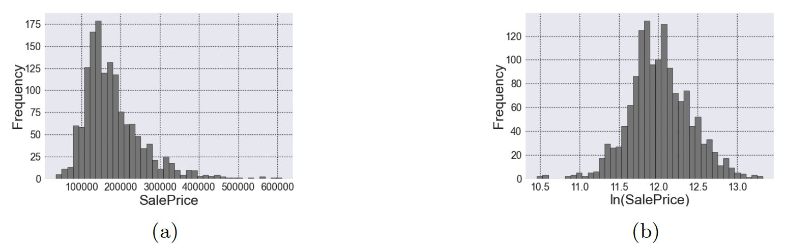
Here, $Q1$ is the column’s first quartile; $Q3$ is the third quartile; and $IQR$ is the column’s interquartile range, given by $Q3-Q1$. Suspected outliers are the datapoints that lie between the inner and outer fences whereas certain outliers are those that exceed the outer fences. To address outliers in the target column (i.e., the ‘Sale Price’ column), we apply a natural log transformation to balance the data and thus make it more suitable for the machine-learning model. Figure 1 shows the histogram for the target column before and after the natural log transformation. Missing values can be handled by looking at the data description provided with the dataset. Table 6 in the Appendix summarizes how the missing variables are handled for each column with missing data.

Figure 1:Histograms of the target column ‘SalePrice’ before (1a) and after (1b) a natural log transformation.

Categorical data can be classified as being either ordinal or nominal. Ordinal data is defined as data with a natural order (e.g., rankings, order or scaling). As a result, we can transform ordinal variables into ordered numbers. For example, the variable column ‘ExterCond’ has 5 possible values: poor, fair, average, good, and excellent. We encode these as follows: poor - 1, fair - 2, average - 3, good - 4, and excellent - 5. Table 7 in the Appendix shows the comprehensive transformations for the 20 ordinal variable columns.

On the other hand, nominal data is defined as data used for naming or labelling purposes. Consequently, nominal data does not have quantitative values or a natural order. Thus, for nominal variables we create “dummy” columns via one-hot encoding as follows: Given a nominal variable column, we create a new dummy column for each possible value determined by the column. Then, for a given property, we mark a ‘1’ to the dummy column corresponding to the property’s variable value, and a ‘0’ for the non-corresponding dummy columns. This process can be further understood by examining Table 1.

Feature Processing

Feature engineering plays an important role in a learning machine model’s success or failure. Feature engineering is the process of extracting new features from raw data. In our model, we create new features by calculating ages and by creating polynomials using variables with a moderate to strong correlation to ‘SalePrice’. Two new features are constructed by calculating the ages ‘GarageAge’ and ‘AgeAtSale’ as follows^[5]:

$$GarageAge = YrSold - GarageYrBlt \tag{5}$$

$$AgeAtSale = YrSold - YearRemodAdd \tag{6}$$

To be sure, we construct these specific variables assuming that age matters in estimating the price of a house. For example, we assume that all else equal, a 10 year old house will have a different price than a 50 year old house with the same features. The same logic applies for the age of a house’s garage.

Now, to determine the features with a moderate to strong correlation to ‘SalePrice’, we calculate Spearman’s rank correlation coefficient $\rho$ (Spearman, 1910). Spearman’s method is preferable as it is able to recognize strong, linear and nonlinear, monotonic relationships. We shall consider only the features with a correlation coefficient greater than 0.50. Let $x$ represent a given feature column and let $y$ represent the target column ‘SalePrice’. The Spearman rank correlation coefficient is calculated similar to the Pearson correlation coefficient,

$$\rho_{rg_x,rg_y}=\frac{Cov(rg_x,rg_y)}{\sigma_{rg_x}\sigma_{rg_y}}$$

where $rg_{x_i}$ is the rank of $x_i$ and $rg_{y_i}$ is the rank of $y_i$. Here, $Cov(rg_x, rg_y)$ is the covariance between $rg_x$ and $rg_y$; $\sigma_{rg_x}$ and $\sigma_{rg_y}$ are the standard deviations of $rg_x$ and $rg_y$, respectively. Table 2 displays the features with a Spearmank rank correlation greater than 0.50. Three new features are then created for each feature^[6] in Table 2 using the equations (7), (8), and (9), where $x$ represents the respective feature:

$$x_{squared} = x^2 \tag{7}$$

$$x_{cubed} = x^3 \tag{8}$$

$$x_{sqrt} = \sqrt{x} \tag{9}$$

Since raw data values often vary widely (e.g., square footage vs number of rooms), we also perform feature normalization and standardization.^[7] First, we normalize strongly skewed numerical features using the one-parameter Box-Cox transformation (Box & Cox, 1964). In order to determine which features are strongly skewed, we calculate the Fisher-Pearson coefficient of skewness (Equations (10) and (11); Pearson, 1894).

$$M_j=\frac{1}{m} \sum_{i=1}^{m} (x_i - \bar{x})^j \tag{10}$$

$$g_1=\frac{M_3}{{M_2}^{\frac{3}{2}}}=\frac{\frac{1}{m} \sum_{i=1}^{m}(x_i-\bar{x})^3}{[\frac{1}{m}\sum_{i=1}^{m}(x_i-\bar{x})^2]^{\frac{3}{2}}} \tag{11}$$

A perfectly symmetric distribution will have a $g_1$ coefficient of 0, or close to 0 if slightly asymmetric; a distribution that is skewed left will have a negative $g_1$ coefficient; and a distribution that is skewed right will have a positive $g_1$ coefficient. The larger the magnitude of $g_1$, the more skewed the data is. For our purposes, we will define strongly skewed features as having a $g_1$ coefficient with an absolute value that is greater than 1. Table 9 in the Appendix displays such features. The one-parameter Box-Cox transformation is then performed as follows where, again, $x$ denotes a given feature:

$$x_i^{(\lambda)}= \begin{cases} \frac{x_i^\lambda-1}{\lambda} & \text{if }\lambda\neq0\text{,} \\ ln(x_i) & \text{if }\lambda=0\text{.} \end{cases} \tag{12}$$

The parameter $\lambda$ is chosen as the optimal parameter to approximate a normal distribution for $x$. Finally, we standardize our features simply as

$$x_{new}=\frac{x_{old}-\bar{x}}{s_x}$$

where $\bar{x}$ and $s_X$ are the feature’s sample mean and sample standard deviation, respectively.

Results & Discussion

To assess the performance of the various kernels, we use the stratified k-fold cross validation technique. Additionally, we use the R-squared score ($R^2$) and the mean absolute error (MAE) to compare the results. These metrics are found by Equations (13) and (14) where $y_i$ is the observed ‘SalePrice’, $\hat{y}_i$ is the predicted price, and $\bar{y}$ is the average observed ‘SalePrice’.

$$R^2 = 1-\frac{\sum_{i=1}^m(\hat{y}_i-\bar{y}_i)^2}{\sum_{i=1}^m(y_i-\bar{y}_i)^2} \tag{13}$$

$$MAE=\frac{1}{m}\sum_{i=1}^m|\hat{y}_i-\bar{y}_i| \tag{14}$$

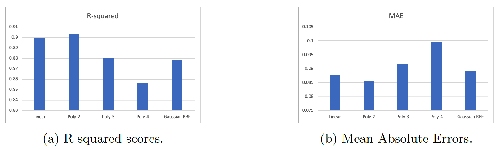
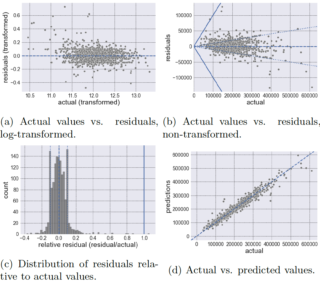
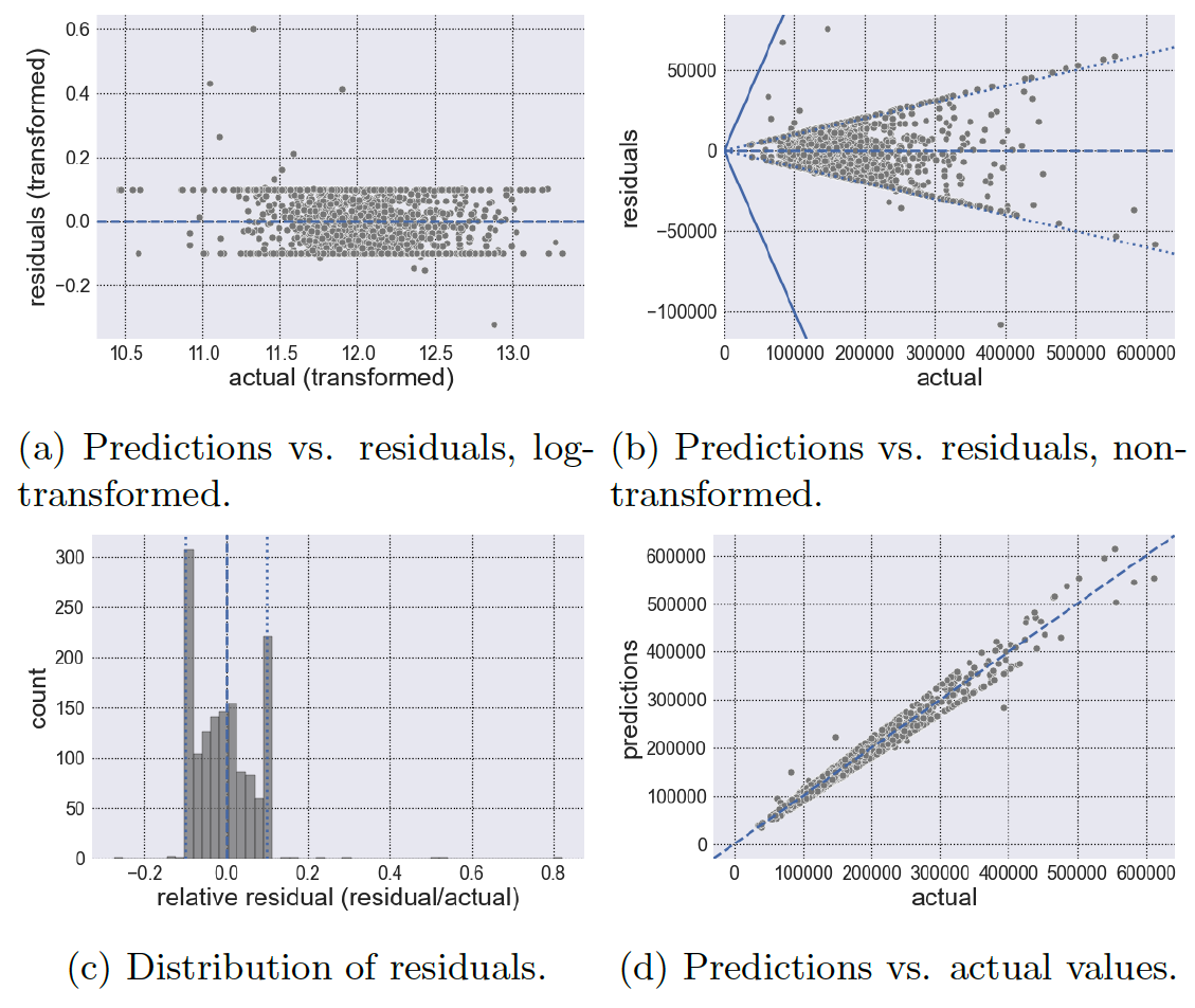
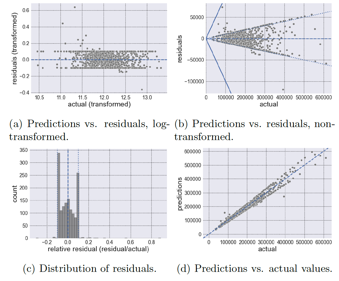
Figures 3 - 7 display the results for each kernel. In each figure, we will show the observed vs. residuals using log-transformed values (a), the observed vs. residuals using the reverted values (i.e., we undo the log transformation) (b), the distribution of residuals relative to the observed values (or $residual/observed$) (c), and finally the actual (i.e., observed) vs. predicted values (d). Also, figures (a), (b) and (d) have a dashed line where $actual=predicted$ so that there is no residual. Moreover, figures (b) have 2 additional lines: one solid and one dotted. The solid line represents a residual value equal to the actual value; therefore anything exceeding the solid lines represents an error larger than the actual value of the house. The dotted line on the other hand, represents a residual value equal to one-tenth of the actual value; anything between the dotted lines represents an error of less than one-tenth of the actual value. Accordingly, anything between the dotted and solid lines would represent an error between 10% and 100% of the actual value. Obviously, a good model would have minimal errors that exceed the dotted line, perhaps no errors beyond the solid line, and maximal errors within the dotted lines. In other words, a good model should have errors/residuals that are small in magnitude relative to the actual value being predicted. (One should be wary of having a large proportion of errors with 1% of the actual value; while this may be a good thing, it can be a sign of an overfitted model). Table 3 summarizes the count that lay within each boundary. Moving on, Figure 2 displays the resulting $R^2$ and MAE of the kernels. Note that a higher $R^2$ and a lower MAE generally indicate a better model performance. Finally, Table 4 displays the summary statistics for the residuals of each kernel. It is important to note that Table 4 is constructed using the absolute value of the residuals.

Figure 2:Resulting $R^2$ (2a) and MAE (2b) for the 5 kernels.

We begin by examining the results of the linear kernel (Figure 3). The linear kernel has an $R^2$ of 0.89920 (2nd highest) and a MAE of 0.08768 (2nd lowest), making it the second best performer in each metric. Figures 3a and 3b suggest inconsistency in the kernel’s residuals. In fact, the linear kernel’s residuals have the highest variation (std. dev. = $12,022.924) of all the kernels according to Table 4. In contrast to the other kernels who have a low relative residual at lower house prices, the linear kernel shows a large relative residual even at these lower prices. Also noteworthy is that the linear kernel has the least predictions within 10% of the actual value (1144 or 79.50%); and it is the only kernel with a prediction larger in magnitude than the actual value (1 or 0.07%). In addition, the linear kernel has by far the most predictions between 10% and 100% of the actual value (294 or 20.43%). In other words, the linear kernel appears to have the largest relative errors in comparison to the other kernels. Looking at the residual summary statistics in Table 4 we see that the linear kernel has the largest residual mean ($11,844.865) as well as the largest maximum residual ($132,108.955). Due to the seemingly contradictory results, we suspect that the linear kernel suffers from model simplicity.

Figure 3:Results for SVR with a linear kernel.

Next, we look at the polynomial kernel of degree $d=2$ (Figure 4). The polynomial of degree $d=2$ (poly-2) kernel performed the best in each metric, having an $R^2$ of 0.90293 and a MAE of 0.08577. Examining Table 3, we find that the poly-2 kernel has the lowest number of predictions within 1% of the actual value. However, we also find that 1226 (or 85.20%) of predictions are within 10% of the actual value, a significant improvement from the linear kernel. Although the poly-2 kernel performs well overall, it also shows an inability in achieving extreme accuracy. Table 3 reveals that the poly-2 kernel had the lowest number of predictions within 1% of the actual value (120 or 8.34%); Table 4 reveals that the poly-2 kernel has the highest minimum error (14.470). Still, though it fails in achieving extreme accuracy in comparison to the other kernels, the poly-2 kernel displays very strong prediction capabilities within a relatively small bound.

Figure 4:Results for SVR with a polynomial kernel of degree d = 2 (poly-2).

Moving forward, we examine the polynomial of degree $d=3$ kernel (Figure 5). The polynomial of degree $d=3$ (poly-3) kernel has an $R^2$ of 0.88023 (3rd highest) and a MAE of 0.09166 (4th lowest), making it a close competitor with the gaussian RBF kernel. The residuals of the kernel appear to behave similar to the residuals from the poly-2 kernel; in fact, the poly-3 kernel has a similar count of residual predictions within 10% (1225 or 85.13%) and between 10% and 100% (213 or 14.80%) of the actual value. However, the poly-3 kernel does appear to be capable of achieving high accuracy; with a count of 129 predictions (8.96%) being within 1% of the actual value; the lowest maximum error ($107,552.218); and a minimum residual ($4.975) significantly lower than that of the poly-2 kernel, though comparable to the other kernels.

Figure 5:Results for SVR with a polynomial kernel of degree d = 3 (poly-3).

Now we examine the polynomial kernel of degree $d=4$ (Figure 6). This kernel has an $R^2$ of 0.85604 (the lowest score) and a MAE of 0.09957 (the highest error), making it the poorest performing kernel according to these metrics. This leads us to suspect that the polynomial of degree $d=4$ (poly-4) kernel is trading off performance for complexity. Indeed, the poly-4 kernel achieves the second highest count of predictions within 1% of the actual value (134 or 9.31%); though it also has the second highest count of predictions between 10% and 100% (242 or 16.82%), behind the linear kernel. Another contradiction is that the poly-4 kernel has the lowest minimum error ($3.054) but also the second highest residual mean ($11,429.242) and the second highest maximum error ($119,033.523), behind the linear kernel. We thus suspect that the poly-4 kernel is suffers from model complexity.

Figure 6:Results for SVR with a polynomial kernel and degree d = 4 (poly-4).

Lastly, we examine the gaussian RBF kernel (Figure 7) which has an $R^2$ of 0.87840 (4th highest) and a MAE of 0.08920 (3rd lowest), resulting in scores comparable to that of the poly-3 kernel. Like the poly-3 and poly-4 kernels, the gaussian RBF kernel is capable of achieving high accuracy, having a count of 142 (9.87%) of predictions with 1% of the actual value. Further, it has the lowest count (205 or 14.25%) of predictions between 10% and 100% of the actual value. Table 4 shows that the kernel has a performance between the poly-3 and poly-4 kernels. Namely, looking at the residual mean ($11,040.674), minimum ($3.174) and maximum ($116,578.736) residuals, the gaussian RBF kernel has metrics higher than the poly-3 kernel though lower than the poly-4 kernel. It is doubtful whether or not this kernel is also suffering from model complexity.

Figure 7:Results for SVR with an Gaussian RBF kernel.

In summary, each kernel achieved favorable results overall. We suspect the linear kernel of under performing due to model simplicity; and the poly-4 kernel (and perhaps the gaussian RBF kernel) of poor generalization due to model complexity. The result being that the poly-2 and poly-3 kernels would be preferable for future house price prediction models. The poly-2 kernel does a good job of predicting house prices overall within a certain boundary, though it fails in achieving a high level of accuracy in comparison to the poly-3 and the more complex models. This could be a generalization issue and should be examined further. On the other hand, the poly-3 kernel does achieve a high level of accuracy but tends to perform slightly worse than the poly-2 kernel overall. Indeed, when comparing the simpler and more complex models, there does appear to exist a trade off between model complexity and performance. Examining figures (a) for each kernel, we see that the log-transformation succeeded in penalizing errors uniformly. That is, the log-transformation’s goal was to maintain relatively equal penalties for both small and large house prices; otherwise, the penalties from large houses would dominate model fitting (since they would tend to be larger in magnitude).

Conclusion

In this paper, we employed a supervised machine-learning model for house price prediction, viz., the SVM for regression estimation (or support vector regression, SVR) model. We also explored 5 different hyper-dimensional mapping kernels: the linear kernel; the polynomial kernel with degrees $d=2, 3, 4$; and the gaussian radial basis function (RBF) kernel. We performed statistical techniques (data cleaning, feature engineering, normalization and standardization) to prepare our data for the SVR model. To reduce over-fitting, we utilized the stratified k-fold cross-validation technique in training and testing our model. Model performance was evaluated using the r-squared score ($R^2$) and the mean absolute error (MAE). Our findings show that the polynomial kernels of degree d=2 and 3 (poly-2 and poly-3) performed the best overall. This may be due to a balance of simplicity and complexity which results in better generalization. Even with limited data on more expensive houses, our models appear to perform relatively well at predicting such house prices. Still, we would like to collect more data at those prices to test for performance improvement.

When constructing machine-learning models, data preparation is just as important as the amount of data available. Even more, the application of statistical analysis in data processing are of paramount importance. In order to improve our models, we might consider exploring additional or even different statistical techniques. As mentioned, we may also want to collect additional data on more expensive houses. (With machine-learning models, however, more data does not always improve performance.) To further test the generalization of our model, we would like to apply it to other house price datasets.