undefined

Introduction

Prior to making a large purchase, many individuals perform online research. This is certainly true for any individual interested in vacationing at a certain locale, during a certain time of year. Taken to its logical next step, a purchaser of a home would most certainly perform their due diligence in gathering as much information as possible regarding the many different amenities of the (potential) geographic location and the many dimensions of the home if a candidate home (or set of homes) has been chosen. One of the least costly methods of gathering information for anyone with access to the internet is the search engine. In this paper, we exploit the vast availability of search query data to find out if the online search behavior which preempts purchasing activity in housing markets can improve the forecasting ability of econometric models.

We demonstrate that incorporating crowd-sourced online search query data into models of the housing market does not improve their forecasting ability. Relative forecasting ability here is the comparison of various performance measures across models which include the search query data versus models where the query data is absent in dynamic, out-of-sample forecasts.^[1]

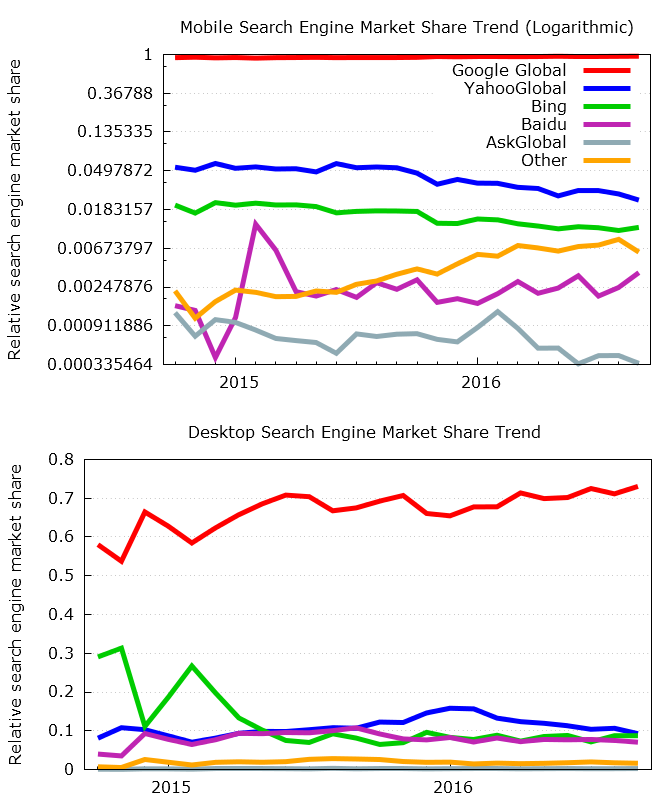
Google Trends is a freely available online tool provided by Google, which has been in operation since 2006. It enables one to input search query terms and it provides a series of data depicting the relative interest in that term by other individuals making similar search queries. The reason we chose Google as the search engine to provide this data is the dominating market share Google occupies in the search engine space. Figure 1 depicts the time series data for Google’s search engine market share in comparison to a handful of other popular search engines.

The plots in figure 1 demonstrate that the data we obtain from Google Trends can be assumed approximately representative owing to the vast majority of search queries on the internet performed using Google. Google’s dominance in the market is most extreme for searches conducted from mobile devices and from tablets. The difference between Google and the other search engines is so vast, the top of figure 1 has been logged in order to allow for the ranking of competing search engines.

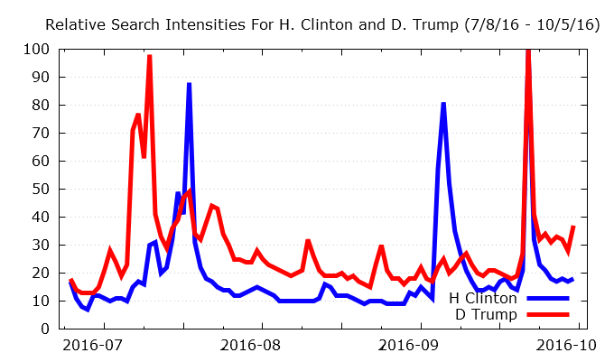
For our readers who may not be familiar with what the information from Google Trends looks like, as a simple example figure 2 shows the time series of search intensity for the two 2016 presidential candidates during the time frame leading up to the first debate.

July turned out to be a very good month for raising contributions for the Trump campaign, while the same bode true for Clinton leading up to August. A different (and perhaps more likely) explanation may be that the spikes in online interest are tied to the uncovering of various scandals and the continual interparty mud-slinging which has riddled this presidential campaign cycle. The first debate occurred on September 26th, which is likely responsible for the concurrent spike in the online interest for both candidates around that time period.

According to the Google Trends help page, the search query data we have retrieved are based on two determinants of the search query: time and location. Every data point in the Google Trends database is computed by dividing the total searches from a specific geographic region and the time period the total searches cover, which results in a relative popularity measure. This resulting number is then scaled on a range from 0 to 100, with 100 representing the most search volume within this specific geographic region during a specific time range. This normalization of data holds significance in that when we look at the search interests over a period of time for a specific search term, it is in fact showing the search interests in this specific term as a proportion of all of the search terms on all of the terms entered into Google search engine, at a specific geographical location within a specific period of time, comparable only to this specific search term. One reason for the normalization of the data, instead of reporting the raw data, originates from the fact that the raw search volume back in 2004 was lower than that in 2016, since less people were utilizing Google in 2004. Therefore, the raw data will fail to capture the relative popularity across time.

In the earlier election example illustrated by figure 2, suppose we add two different time series of Google Data Trends data on the search terms for “Hillary Clinton” and “Donald Trump” into one timeframe at the same geographic location. Then adding another fairly irrelevant search term, such as “pumpkin” will not affect the Google Trends data because the normalized search index for each of these three search terms are first divided by the same denominator, namely the total search volume from the same geographical location during the same time period, and then each data point for a specific search term (e.g. Hillary Clinton) is normalized across all of the computed data points of this specific term (Hillary Clinton). Therefore, we see that although all search terms are divided by the same base, the search index for every term is not comparable across different terms.

The housing price data we will be testing our models against is the S&P/Case-Shiller 20-City Composite Home Price Index provided by FRED. We then take the Metropolitan Statistical Area (MSA) city-level data on housing sales available on Zillow’s data page and weigh the data in accordance with the weighing scheme outlined by the Case-Shiller 20 city housing index.^[2] We follow the same steps in creating the series for online search queries: Google provides the trend data at the city-level and this allows us to to create a national data series on Google Trends which is consistent with the weighing of our sales data and the Case-Shiller index. Since Google Trends data is available from January 2004 through 2016, all of our data series begin on January 2004. In all of the empirical exercises, we split the dataset into a training period and a (out of sample) forecast period. All of the forecasts are performed out of sample as dynamic, one-step-ahead forecasts and evaluated using a root mean-squared deviation metric.

We estimate a baseline linear model following previous studies in the literature. We then re-estimate the model including the Google Trend data. We find that adding the Google Trend data as an explanatory variable in our baseline training/testing period insignificantly improved the performance of the forecast, decreasing the root mean squared deviation from 6.7576 to 6.7483 (decrease of 0.14%) and decreasing the mean absolute percentage error from 96.201 to 94.565. In a robustness check, repeating the exercise with a shorter and longer training window both deteriorate the forecast performance with the RMSD increasing by 0.314% and the MAPE increasing from 109.75 to 111.23 for the shorter training window and the RMSD increasing by 1.425% and the MAPE increasing from 158.68 to 161.14 for the longer training window.

Related literature

This paper builds upon and contributes to a growing body of work which seeks to exploit and/or investigate the predictive power of online search queries in forecasting the future values of various assets.

Beracha & Wintoki (2013) examine whether abnormal housing price changes in a city can be predicted by abnormal search intensity for real estate terms in that specific city. By arguing that search intensity for real estate terms for a specific city can be treated as a proxy for housing market sentiment for that city, Beracha and Wintoki run a regression of abnormal home price changes on the lagged abnormal search intensity for the search terms “real estate” and “rent” for each Metropolitan Statistical Area (MSA) in their sample. They discover that, by using search intensity for real estate terms as a proxy for housing sentiment, abnormal search intensity for real estate terms in a specific city can help predict abnormal future housing price changes. They also find that the predictions for cities with abnormally high search intensity outperform the predictions for cities with abnormally low real estate search volume by as much as 8.5% over a two-year period.

Askitas (2016) creates a buyer-seller index based on the ratio of Google Trends home “buy” queries to home “sell” queries. The index correlates with the SP/Case-Shiller Home Price Index and makes for a fairly decent method to now-cast home prices. Our focus is a bit different as we are testing the out-of-sample forecasting ability with and without online query data and we are also including both past prices and actual housing sales volumes provided by Zillow as independent variables in our models.

Vosen & Schmidt (2011) intend to check how indicators from Google Trend search terms perform when compared to two traditional survey-based indicators, the University of Michigan Consumer Sentiment Index (MCSI) and the Conference Board Consumer Confidence Index (CCI), in forecasting private consumption. Vosen & Schmidt (2011) form a baseline model with MA(1) process and augment the model by adding the MCSI, CCI and Google factors into the model. They then conduct both in-sample and out-of-sample forecasting and find consistent results in supporting Google data as the superior data source for predicting private consumption during their testing period from January 2005 to September 2009.

Finally, additional empirical papers which demonstrate some evidence of the fore- and now-casting power of Google data for specific macroeconomic variables include D’Amuri & Marcucci (2012) (forecasting the unemployment rate), Coble & Pincheira (2017) (now-casting building permits) and Nymand-Andersen & Pantelidis (2018) (now-casting car sales).

Empirical methodology

We estimate a simple set of time series regressions (including and excluding the Google data) and then perform an out-of-sample forecast. We then compare the out-of-sample forecasts with the actual Case-Shiller HPI. We then calculate and provide several measures of forecast performance statistics to compare the models with. For all statistical exercises, the training block spans August of 2004 through December of 2012; we will be testing the forecasting ability of the resulting estimated models on the remaining data which spans January of 2013 through August of 2016. For robustness, we repeat the exercise using a smaller (August 2004 – July 2010) and larger (August 2004 – July 2014) training period.^[3]

Data description

Case-Shiller Home Price Index

Based on the work of Karl Case, Robert Shiller and Allan Weiss, The S&P CoreLogic Case-Shiller Home Price Index Series are “the leading measures of U.S. residential real estate prices, tracking changes in the value of residential real estate both nationally as well as in 20 metropolitan regions.”^[4] The three major indices included in the series are Case-Shiller 20-City Composite Home Price Index, the Case-Shiller 10-City Composite Home Price Index, and the Case-Shiller U.S. National Home Price Index. For the purpose of our research, which focuses on the housing market at the national level, we select the Case-Shiller 20-City Composite Home Price Index for its coverage of 20 significant housing markets in the U.S. at the city level.

A detailed list of the 20 cities included in the composite is presented in table 1.

In order to create the Google search query index that we use to conduct our study, we weigh the city-level Google search query data using the exact same weights as the Case-Shiller. Again, our aim is to remain as consistent as possible when marrying the housing and search query data.

Google Trends Data

Google Trends is a search queries database provided by Google and it has been made available to the general public since its official launch on May 11, 2006, with data going back to as early as 2004. Google Trends provides users with a normalized search intensity index ranging from 0 to 100, with zero indicating no or very little search activity on a specific search term and 100 indicating the highest. Because of data normalization, the user cannot get the exact search intensity amount outside of the context of all search queries submitted to Google Search within a certain period of time. However, the service does provide a convenient data source for comparing the changes in the search intensity for a specific search term over a long period of time. In addition, Google Trends also offers users the option to filter the data at the national, regional or geographical level.

There have been numerous papers written which explore the predictive power of Google Trends data with many researchers having found affirmative results showing that Google Trends data can be utilized to predict near-future events. For example, Choi & Varian (2012) use search engine data from Google to forecast near-term macroeconomic indicators like automobile sales, unemployment claims, and consumer confidence, concluding that “simple seasonal AR models that include relevant Google Trends variables tend to outperform models that exclude these predictors by 5% to 20%.”

To incorporate Google Trends data into our research, we aim to construct a monthly “Google Trends Case-Shiller” search intensities index series for the housing market. To do so, we gather, subject to data availability, Google Trends data for search terms similar to the search semantic “[city] Real Estate Agency”, where “[city]” is all city choices coming from the Case-Shiller 20-City Composite Index (in table 1). We chose “Real Estate Agency” as this search term provided the best result.

As a robustness check, we also re-ran all of the exercises with the default Google “Real Estate” search term and again with the default Google “Real Estate Agency” search term. The search query “Real Estate Agency” provided better results than “Real Estate”, however both resulted in inferior results when compared to the query including the city name.

The available data for the search terms are dated from December 2003 to August 2016 at the monthly frequency. Then to transform these data into our monthly “Google Trends Case-Shiller” search intensities index series, we assign the same weighting scheme from the Case-Shiller 20-City Composite Index (in table 1) to each city’s Google Trends index data and obtain a “Google Trends Case-Shiller” housing search term index for all sets of data across 20 cities.

Zillow Housing Data

Founded in 2006, Zillow is an online real estate database that has more than 110 million U.S. homes, including homes for sale, homes for rent and homes not currently on the market, on its record.^[5] Besides its website, Zillow also offers mobile apps across all mainstream platforms and the popularity among users gives Zillow first-hand data in the real estate market. Zillow releases housing market data periodically on its website and the data are freely accessible by the public.

In order to remain consistent with the Google Trend data, we turn to Zillow in order to create a monthly “Housing sales - Case-Shiller” index. To do this, we obtain the set of sales data at the city level from Zillow and assign each city’s sales data the same weights from table 1. The resulting weighted time series data for sales was trimmed to cover August 2004 to August 2016 at the monthly frequency in order to accommodate the span of Google Trend data we managed to obtain.

Preparation of Data

Prior to any transformation of the data series, all data was seasonally adjusted using X-12 ARIMA. We define our primary variable of interest “house price inflation” as

$$\pi_t = \frac{HPI_t}{HPI_{t-12}} - 1, \tag{1}$$
where $HPI$ is the Case-Shiller housing price composite. The remaining data, made up of the housing sales and Google Trend data (both Case-Shiller weighted), has been stationarized by first differences.^[6] Table 2 reports the results for unit-root ADF and KPSS tests^[7] for all of the variables.

The test results in table 2 point out that there is no evidence (to the 3% level) of a unit-root in any of the time series data we will be using in the econometric exercises.

Estimation

We proceed by breaking the data set into a training block and a testing block. The training set will cover August of 2004 through December of 2012, and the testing data will span the remainder of the set from January 2013 through August of 2016.^[8] We will be formulating an AR model for the Case-Shiller HPI, which also has differenced (Case-Shiller weighted) housing sales and differenced (Case-Shiller weighted) Google search query data as regressors. In order to establish a benchmark, we initially estimate a model excluding the search query data.

Without Google

Following a battery of various combinations, the model we chose as “best”^[9] is

$$\pi_t = \alpha_1\pi_{t-1} + \alpha_2\pi_{t-2} + \alpha_3 dHS_{t-1} + \alpha_4 dHS_{t-2} + \epsilon^{\pi}_t, \tag{2}$$
where $\pi$ is the Case-Shiller HPI and $dHS$ represents differenced (Case-Shiller weighted) housing sales. In choosing the most parsimonious model, we compared the results across three main criterion:

1. appropriateness of the variables chosen in line with our priors as to what the data-generating process for housing price inflation should look like,^[10]

2. the model which minimizes the (negative) of the log-likelihood, while

3. eliminating all of the auto-correlation and partial auto-correlation in the resultant residual series.

The estimation results are reported in table 3.

Both of the autoregressive lags are statistically significant at the 1% level, hinting that aggregate real estate prices exert extreme levels of inertia; differenced housing sales are significant at the 10% level, with sales lagged two periods being significant at the 1% level, demonstrating that past home sales are also indicative of current price movements. The high level of inertia in aggregated housing markets is well known in the literature; Case & Shiller (1989, 1990) studied the high level of persistence in the rate of change of prices, concluding that this was one of the reasons that the housing market remains inefficient.^[11]

With Google

We follow the same procedure in isolating best econometric model when incorporating the Google Trend data as we did in choosing the model without the search query data (The model given by equation (2)). The resultant regression specification is

$$\begin{align} \pi_t = &\alpha_1\pi_{t-1} + \alpha_2\pi_{t-2} + \alpha_3 dHS_{t-1} + \alpha_4 dHS_{t-2} \\ &+ \alpha_5\widehat{\Gamma}_{t-3} + \alpha_6\widehat{\Gamma}_{t-4} + \epsilon^{\pi}_t, \end{align} \tag{3}$$
where variables are as defined before ($\pi$ is the Case-Shiller HPI, $dHS$ represents differenced housing sales) and $d\Gamma$ represents the differenced " Real Estate Agency" Google search queries. This resultant model illustrates that significant deviations in search activity manifest themselves as real movements in the housing market approximately 3 to 4 months later.^[12] The estimation results are reported in table 4.

According to the estimates in table 4, lagged prices and housing sales once again play an important role in the pricing process, however, while online search queries slightly improve the overall fit of the model (according to the log-liklihood of the estimate), both coefficients on search queries are only significant at the 16% level.

Forecasting results for both models

Figure 3 offers a visual representation of how well both models perform out of sample. Actual data contain squares while forecasted data contain triangles. Also included are 95 percent confidence bands on the out-of-sample forecasts.

Table 5 lists two sets (with and without the Google search query data) of forecast performance measures.

Discussion of results

Two meaningful statistical measures presented by table 5 are the Root Mean Squared Deviation $RMSD$ and the Mean Absolute Percentage Error. The root mean squared deviation $RMSD$, is defined as

$$RMSD = \sqrt{\frac{\sum_{t=1}^n\left(\widehat{Data}^F_t - \widehat{Data}^A_t\right)^2}{n}}, \tag{4}$$
where $n$ represents the number of observations in the out-of-sample observations, a superscript $F$ represents “forecasted” and a superscript $A$ represents “actual”. According to table 5, incorporating Google Trends data into the forecast only slightly improves the deviation from 6.7576 to 6.7483, leaving the impression that the crowd-sourced query data doesn’t really add any value to the forecasting ability of the model.

Comparing the Mean Absolute Percentage Error in the forecasts further corroborates the unremarkable performance of the forecast which implements the Google Trend data over the baseline model’s forecast (96.201% baseline compared to 94.565% for the model with Google). In order to test the robustness of these results, we repeated the experiment utilizing a shorter training window^[13] and then once again repeated the experiment utilizing a longer training window.^[14] Unlike the results provided in table 5, in both robustness checks, the performance statistics actually deteriorated when incorporating the Google Trend data; numerical specifics provided in the appendix.

The inefficiency of the housing market has served as a focal point in the literature (Case & Shiller, 1990; Hjalmarsson & Hjalmarsson, 2009), so our prior, based largely on the results from the other studies which incorporated the search query data, was that the Google Trend data would be a promising addition to ARIMA models used to forecast prices in the housing market. However, the empirical tests we have conducted do not provide any proof that the search query data aids in forecasting out-of-sample.

Concluding remarks

In this study, we have answered the research question of whether or not incorporating Google Trends data into models of the housing market actually improves their out-of-sample forecasting ability. The motivation for this study comes from the present trend towards utilizing search query data in empirical economics.

According to our results, incorporating Google Trends does not significantly improve the models’ ability to forecast out-of-sample. While many related papers in the literature (Beracha & Wintoki, 2013; Vosen & Schmidt, 2011) incorporate the same type of search query data in their models and demonstrate statistical significance among the search query regressors, we took this method one step further: does this help in any way when it comes to the ability of these models to forecast out-of-sample? Our conclusion is that the evidence simply does not support this.

These results motivate two follow-up research questions: why is it that incorporating the Google Trend data deteriorate the forecasting ability, and would different types of forecasting tests - such as a dynamic/rolling window forecast, for example - actually provide different results/buttress support for inclusion of the search query data? Would augmenting larger economic models of the housing market provide different results? This is probably unlikely, given the results of Wickens (2014), and also the reputation larger DSGE models have when it comes to their lackluster performance in forecasting macroeconomic data out-of-sample. A separate study involving a theoretical model which can then be estimated in order to make empirical forecasts would be a more appropriate venue to undertake this question; this would be one potential future extension of this work.

---

Appendix

Dynamic forecasting

If we have the following sample AR(1) model

$$y_t = \beta_0 + \beta_1y_{t-1} + \epsilon_t. \tag{5}$$
and we want to forecast $y$ for period $\tau$ and data for $y$ up to period $\tau - 1$ is available, we could estimate
$$\widehat{y}_\tau = \widehat{\beta}_0 + \widehat{\beta}_1\widehat{y}_{\tau-1}. \tag{6}$$
Now assume that only the data up until period $\tau - 2$ is available so that we estimate
$$\widehat{y}_{\tau - 1} = \widehat{\beta}_0 + \widehat{\beta}_1\widehat{y}_{\tau-2}. \tag{7}$$
Then we can take our estimate for $\widehat{y}_{\tau - 1}$ from (7) and feed this in for $\widehat{y}_{\tau - 1}$ in (6). The result is what we refer to as a dynamic forecast.

Shorter training window

Tables 6 and 7 show the regression results for two other combinations of training/forecasting periods.

Table 8 contains out-of-sample performance measures for two other combinations of training/forecasting periods.

Longer training window

Table 11 contains out-of-sample performance measures for a longer training/shorter forecasting period.

---

1. For readers unfamiliar with dynamic forecasting, refer to the appendix for an explanation. Examples of time series forecast performance measures include (R.M.S.D.) root mean squared deviation, (M.A.P.E.) mean absolute percentage error, etc.

2. The data were freely available up until 2017, when Zillow changed their policies regarding the availability of their data. The data is no longer free; we thus chose to only include the data in this study that were freely available at the time. As a result, our raw data files span 2004 - 2016.

3. These results are provided in the appendix.

4. http://us.spindices.com/index-family/real-estate/sp-corelogic-case-shiller

5. http://www.zillow.com/corp/About.htm

6. An HP-filtered set of time series data is not appropriate for this type of analysis; since the HP-filter is two-sided and this is an exercise in testing forecasting ability, at the forecast point the filter would rely on data which hasn’t arrived.

7. ADF is the acronym for the Augmented Dickey-Fuller test and KPSS is the acronym for the Kwiatkowski–Phillips–Schmidt–Shin test.

8. Robustness results using smaller and larger training windows provided in the Appendix.

9. The model we chose also takes on the same structure as in Wu & Brynjolfsson (2015).

10. For example, it is well known that housing prices exhibit a fair amount of persistence, and housing sales typically contribute to housing price inflation with a slight lag; the resultant model fits this prior.

11. While city-wide indexes (similar to ours in the current study) exhibit persistence, forecasting excess returns at the individual house level remains difficult due to the relatively high level of noise in individual prices.

12. According to homes.com, for the average home buyer, the process from shopping to first mortgage payment can take anywhere from 2 to 6 months. This doesn’t take into account the early online research stages conducted by most potential buyers.

13. 2005:08–2010:07 ($T$ = 60) compared to 2005:08–2012:12 ($T$ = 89).

14. 2005:08–2014:07 ($T$ = 108) compared to 2005:08–2012:12 ($T$ = 89).